TABLE OF CONTENTS

types of data

Discrete data, as the name suggests, can take only specified values. For example, when you roll a die, the possible outcomes are 1, 2, 3, 4, 5 or 6 and not 1.5 or 2.45.

Continuous data can take any value within a given range. The range may be finite or infinite. For example, A girl’s weight or height, the length of the road. The weight of a girl can be any value from 54 kgs, or 54.5 kgs, or 54.5436kgs.

types of distributions

Bernoulli distribution

A Bernoulli distribution has only two possible outcomes, namely 1 (success) and 0 (failure), and a single trial.

$P(x) = \begin{cases} 1 - p& x = 0 \\ p & x = 1 \end{cases}$

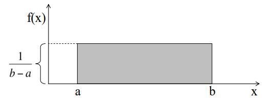
Uniform distribution

When you roll a fair die, the outcomes are 1 to 6. The probabilities of getting these outcomes are equally likely and that is the basis of a uniform distribution. Unlike Bernoulli Distribution, all the n number of possible outcomes of a uniform distribution are equally likely.

Uniform distribution if:

$f(x) = \frac{1}{(b-a)}$

for

$-\infty < a \leq x \leq b < \infty$

Binomial Distribution

lorem ipsum

Normal Distribution

lorem ipsum

Poisson Distribution

lorem ipsum

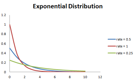
Exponential Distribution

"interpretations" of probability

Bayesian probability

Bayesian probability is an interpretation of the concept of probability, in which, instead of frequency or propensity of some phenomenon, probability is interpreted as reasonable expectation representing a state of knowledge or as quantification of a personal belief.

an extension of propositional logic that enables reasoning with hypotheses

Quantum Bayesianism

Quantum Bayesianism (abbreviated QBism, pronounced "cubism") is an interpretation of quantum mechanics that takes an agent's actions and experiences.

This interpretation is distinguished by its use of a subjective Bayesian account of probabilities to understand the quantum mechanical Born rule as a normative addition to good decision-making.

Born rule

The Born rule (also called the Born law, Born's rule, or Born's law), formulated by German physicist Max Born in 1926, is a physical law[citation needed] of quantum mechanics giving the probability that a measurement on a quantum system will yield a given result. In its simplest form it states that the probability density of finding the particle at a given point is proportional to the square of the magnitude of the particle's wavefunction at that point. The Born rule is one of the key principles of quantum mechanics.

history of quantum probability

The old quantum theory is a collection of results from the years 1900–1925 which predate modern quantum mechanics. The theory was never complete or self-consistent, but was rather a set of heuristic corrections to classical mechanics. The theory is now understood as the semi-classical approximation to modern quantum mechanics.

Where the ${\displaystyle p_{i}}$ are the momenta of the system and the ${\displaystyle q_{i}}$ are the corresponding coordinates. The quantum numbers ${\displaystyle n_{i}}$ are integers and the integral is taken over one period of the motion at constant energy (as described by the Hamiltonian). The integral is an area in phase space, which is a quantity called the action and is quantized in units of Planck's (unreduced) constant. For this reason, Planck's constant was often called the quantum of action.

events that led to quantum theory:

• In his 1905 paper on light quanta, Einstein created the quantum theory of light. His proposal that light exists as tiny packets (photons) was so revolutionary, that even such major pioneers of quantum theory as Planck and Bohr refused to believe that it could be true. Bohr, in particular, was a passionate disbeliever in light quanta, and repeatedly argued against them until 1925, when he yielded in the face of overwhelming evidence for their existence.
• In 1905, Einstein noted that the entropy of the quantized electromagnetic field oscillators in a box is, for short wavelength, equal to the entropy of a gas of point particles in the same box. The number of point particles is equal to the number of quanta. Einstein concluded that the quanta could be treated as if they were localizable objects, particles of light, and named them photons.
  • Einstein's theoretical argument was based on thermodynamics, on counting the number of states, and so was not completely convincing. Nevertheless, he concluded that light had attributes of both waves and particles, more precisely that an electromagnetic standing wave with frequency ${\displaystyle \omega }$ with the quantized energy:
  • ${\displaystyle E=n\hbar \omega \,}$
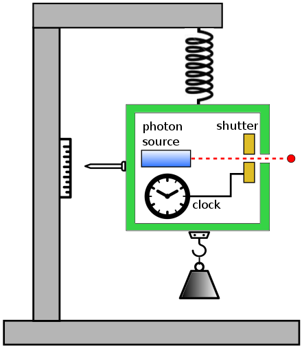
• Einstein proposed the wave-particle duality of light. In 1909, using a rigorous fluctuation argument based on a thought experiment and drawing on his previous work on Brownian motion, he predicted the emergence of a "fusion theory" that would combine the two views. Basically, he demonstrated that the Brownian motion experienced by a mirror in thermal equilibrium with black body radiation would be the sum of two terms, one due to the wave properties of radiation, the other due to its particulate properties.
• In 1913, Niels Bohr identified the correspondence principle and used it to formulate a model of the hydrogen atom which explained the line spectrum.

biggest concepts:

• light quanta
• wave-particle duality
• the fundamental randomness of physical processes
• the concept of indistinguishability
• the probability density interpretation of the wave equation

Axiomatic probability

The mathematics of probability can be developed on an entirely axiomatic basis that is independent of any interpretation:

probability theory

probability axioms

first:

probability of an event is a non-negative real number:

${\displaystyle P(E)\in \mathbb {R} ,P(E)\geq 0\qquad \forall E\in F}$

where ${\displaystyle F}$ is the event space. It follows that ${\displaystyle P(E)}$ is always finite, in contrast with more general measure theory. Theories which assign negative probability relax the first axiom.

second:

assumption of unit measure: that the probability that at least one of the elementary events in the entire sample space will occur is 1

third:

Any countable sequence of disjoint sets (synonymous with mutually exclusive events) ${\displaystyle E_{1},E_{2},\ldots } {\displaystyle E_{1},E_{2},\ldots }$ satisfies

$P\left(\bigcup _{i=1}^{\infty }E_{i}\right)=\sum _{i=1}^{\infty }P(E_{i}).$

axiomatic consequences

The probability of the empty set.

${\displaystyle P(\varnothing )=0}$

In some cases, ${\displaystyle \varnothing }$ is not the only event with probability ${\displaystyle 0}$.

Monotonicity

${\displaystyle \quad {\text{if}}\quad A\subseteq B\quad {\text{then}}\quad P(A)\leq P(B)}$.

If A is a subset of, or equal to B, then the probability of A is less than, or equal to the probability of B.

numeric bound

It immediately follows from the monotonicity property that

${\displaystyle 0\leq P(E)\leq 1\qquad \forall E\in F}$

addition law of probability

$P(A\cup B)=P(A)+P(B)-P(A\cap B)$

coin toss

$\Omega =\{H,T\}$

${\displaystyle F=\{\varnothing ,\{H\},\{T\},\{H,T\}\}}$

Kolmogorov's axioms imply that:

$P(\varnothing )=0$

The probability of neither heads nor tails, is 0.

${\displaystyle P(\{H,T\}^{c})=0}$

The probability of either heads or tails, is 1.

$P(\{H\})+P(\{T\})=1$

resources, links, notes

• Probability axioms - Wikipedia
• 6 Probability Distributions every data science professional should know

Share the love!

Thank y'all kindly for the read!